The goals / steps of this project are the following:
- Perform a Histogram of Oriented Gradients (HOG) feature extraction on a labeled training set of images and train a classifier Linear SVM classifier
- Optionally, you can also apply a color transform and append binned color features, as well as histograms of color, to your HOG feature vector.
- Note: for those first two steps don't forget to normalize your features and randomize a selection for training and testing.
- Implement a sliding-window technique and use your trained classifier to search for vehicles in images.
- Run your pipeline on a video stream (start with the test_video.mp4 and later implement on full project_video.mp4) and create a heat map of recurring detections frame by frame to reject outliers and follow detected vehicles.
- Estimate a bounding box for vehicles detected.
The code for this step is contained in the "Get HOG features" code cell of the IPython notebook Vehicle detection and tracking.ipynb.
I started by reading in all the vehicle and non-vehicle images. Here are a few images from vehicle and non-vehicle classes:

I then explored different color spaces and different skimage.hog() parameters (orientations, pixels_per_cell, and cells_per_block). I grabbed random images from each of the two classes and displayed them to get a feel for what the skimage.hog() output looks like.
The figure below shows a comparison of a car image and its associated HOG features, as well as the same for a non-car image.
The method extract_features() accepts a list of image paths and HOG parameters and produces a flattened array of HOG features for each image in the list.

I tried various combinations of colorspaces X orientations X Pixels per cell X Cells per block X HOG channels and settled on the final choice based on the performance of SVC classifier produced using them.
The final parameters I used are documented below:
- colorspace = 'YUV'
- orient = 11
- pix_per_cell = 16
- cell_per_block = 2
- hog_channel = 'ALL'
As done in the "Train a Classifier" code cell, a Support Vector Classifier is trained on 80% of the dataset to produce an accuracy of 98.28% on 20% of the remaining dataset (test set).
I used the method find_cars() from the lesson materials. The method combines HOG feature extraction with a sliding window search, but rather than perform feature extraction on each window individually which can be time consuming, the HOG features are extracted for the entire image (or a selected portion of it) and then these full-image features are subsampled according to the size of the window and then fed to the classifier. The method performs the classifier prediction on the HOG features for each window region and returns a list of rectangle objects corresponding to the windows that generated a positive ("car") prediction.
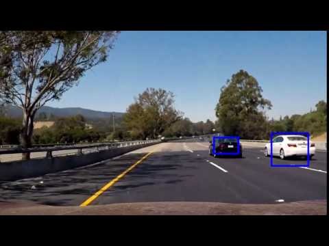
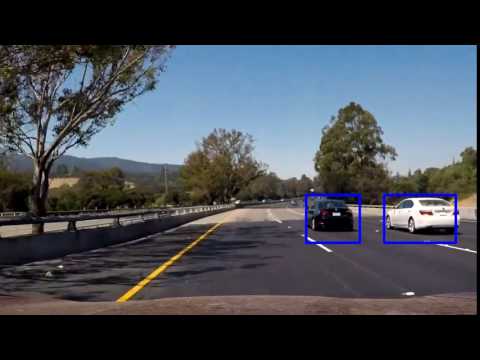
I explored several configurations of window sizes and positions, with various overlaps in the X and Y directions. Small scales (<0.8) returned too many false positives so scales of 1 and above were used. The window scale and start/stop positions finally used are described in "Combine Various Sliding Window Searches" of the notebook. The image below shows the rectangles returned by find_cars drawn onto one of the test images in the final implementation.

The add_heat function increments the pixel value (referred to as "heat") of an all-black image the size of the original image at the location of each detection rectangle. Areas encompassed by more overlapping rectangles are assigned higher levels of heat. The following image is the resulting heatmap from the detections in the image above:

A threshold is applied to the heatmap (in this example, with a value of 1), setting all pixels that don't exceed the threshold to zero. The result is below:

The scipy.ndimage.measurements.label() function collects spatially contiguous areas of the heatmap and assigns each a label:

And the final detection area is set to the extremities of each identified label:


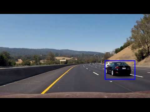
The final implementation performs reasonably well with no false positives in the test images.
The first implementation did not perform as well, so I began by optimizing the SVM classifier. Initially, the classifier used HOG features from the YUV Y channel only, and achieved a test accuracy of 96.28%. Using all three YUV channels increased the accuracy to 98.2%.
Other optimization techniques included changes to window sizing and overlap as described above, and lowering the heatmap threshold to improve accuracy of the detection.
The following videos show different stages of progress made with the approach.
Following is the output when each frame is processed independently:
Rather than performing the heatmap/threshold/label steps for the current frame's detections, the detections for the past 15 frames are combined and added to the heatmap and the threshold for the heatmap is set 8.5 - this value was found to perform best empirically.
The following video shows the results of combining information across the frames:
And below is the final project video:
It was a good experience to learn about the sliding window method. I noticed that it has a couple of disadvantages - The most important one being that it is computationally very expensive. It requires so many classifier tries per image. Again for computational reduction not whole area of input image is scanned. So when road has another placement in the image like in strong curved turns or camera movements, sliding windows may fail to detect cars.
The Single Shot MultiBox Detector might be a good alternative for the sliding windows approach.